The goal of touringplans is to provide access to Disney World Ride Wait Time Datasets curated by the TouringPlans.com team.
Installation
You can install the development version of touringplans with:
devtools::install_github("LucyMcGowan/touringplans")You can find a list of all data sets along with variable information on the touringplans package website
Example
The touringplans_2018 data frame contains wait time data aggregated by hour for 14 attractions, along with some park-level daily metadata. The example below demonstrates how wait times by day are associated with the Ticket Season. The example below uses the tidyverse package to assist with data wrangling.
library(touringplans)
library(tidyverse)
touringplans_2018 %>%
  count(attraction_name)
#> # A tibble: 14 × 2
#>    attraction_name                                           n
#>    <chr>                                                 <int>
#>  1 Alien Swirling Saucers                                 2718
#>  2 Avatar Flight of Passage                               5147
#>  3 DINOSAUR                                               4884
#>  4 Expedition Everest - Legend of the Forbidden Mountain  4950
#>  5 Kilimanjaro Safaris                                    4887
#>  6 Na'vi River Journey                                    5073
#>  7 Pirates of the Caribbean                               5168
#>  8 Rock 'n' Roller Coaster Starring Aerosmith             5062
#>  9 Seven Dwarfs Mine Train                                5622
#> 10 Slinky Dog Dash                                        2691
#> 11 Soarin' Around the World                               5203
#> 12 Spaceship Earth                                        5078
#> 13 Splash Mountain                                        4964
#> 14 Toy Story Mania!                                       5045
We can aggregate the hourly posted wait time data into an avarage wait time by day for each ride.
agg_2018 <- touringplans_2018 %>%
  group_by(park_date, attraction_name, park_ticket_season) %>%
  summarise(average_diff = mean(wait_minutes_posted_avg - wait_minutes_actual_avg, na.rm = TRUE), .groups = "drop") %>%
  filter(average_diff > -300) # remove weird data points (more on this later!)
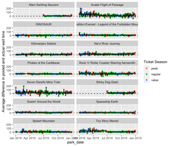
On average, Disney over predicts wait times by 15 and a half minutes per day on the 14 rides included in this dataset during peak season, around 11 and a half minutes per day during regular season, and around 13 minutes per day during value season.
lm(average_diff ~ park_ticket_season, data = agg_2018) %>%
  summary()
#>
#> Call:
#> lm(formula = average_diff ~ park_ticket_season, data = agg_2018)
#>
#> Residuals:
#>     Min      1Q  Median      3Q     Max
#> -82.401  -8.734  -3.066   5.487 198.772
#>
#> Coefficients:
#>                           Estimate Std. Error t value Pr(>|t|)
#> (Intercept)                15.6420     0.6006  26.045  < 2e-16 ***
#> park_ticket_seasonregular  -3.9076     0.7074  -5.524 3.53e-08 ***
#> park_ticket_seasonvalue    -2.4144     0.8378  -2.882  0.00397 **
#> ---
#> Signif. codes:  0 '***' 0.001 '**' 0.01 '*' 0.05 '.' 0.1 ' ' 1
#>
#> Residual standard error: 17.57 on 3967 degrees of freedom
#> Multiple R-squared:  0.007723,   Adjusted R-squared:  0.007223
#> F-statistic: 15.44 on 2 and 3967 DF,  p-value: 2.095e-07
ggplot(agg_2018, aes(x = park_date, y = average_diff)) +
  geom_point(aes(color = park_ticket_season)) +
  geom_line() +
  geom_hline(yintercept = 0, lty = 2) +
  facet_wrap(~ attraction_name, ncol = 2) +
  labs(y = "Average difference in posted and actual wait time",
       color = "Ticket Season")
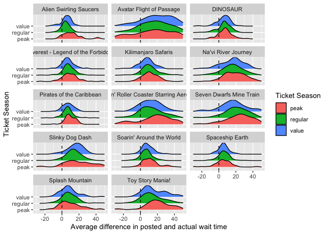
We can see that there are some attractions that this holds true for moreso than others.
library(ggridges)

ggplot(agg_2018, aes(x = average_diff, y = park_ticket_season, fill = park_ticket_season)) +
  geom_density_ridges() +
  geom_vline(xintercept = 0, lty = 2) +
  xlim(c(-30, 50)) +
  facet_wrap(~ attraction_name, ncol = 3) +
  labs(x = "Average difference in posted and actual wait time",
       fill = "Ticket Season",
       y = "Ticket Season")