The Whole Game
- Specify causal question (e.g. target trial)
- Draw assumptions (causal diagram)
- Model assumptions (e.g. propensity score)
- Analyze propensities (diagnostics)
- Estimate causal effects (e.g. IPW)
- Sensitivity analysis (tipping points)
We’ll focus on the broader ideas behind each step and what they look like all together; we don’t expect you to fully digest each idea. We’ll spend the rest of the class taking up each step in detail
Does using a bed net reduce the risk of malaria?
Malaria and its Impact
- Malaria remains a significant public health concern
- Six countries (Nigeria, DRC, Uganda, Mozambique, Angola, Burkina Faso) saw nearly 50% of all malaria deaths
- Most fatalities happened among children under 5
Role of Bed Nets
- Bed nets are vital in preventing malaria
- They create a barrier against mosquito bites, the main carriers of malaria parasites
- Several randomized studies have shown that bed nets reduce the risk of malaria
Historical Use of Bed Nets
Herodotus noted Egyptians using fishing nets as bed nets in the 5th century BC
Against the gnats, which are very abundant, they have contrived as follows:—those who dwell above the fen-land are helped by the towers, to which they ascend when they go to rest; for the gnats by reason of the winds are not able to fly up high: but those who dwell in the fen-land have contrived another way instead of the towers, and this is it:—every man of them has got a casting net, with which by day he catches fish, but in the night he uses it for this purpose, that is to say he puts the casting-net round about the bed in which he sleeps, and then creeps in under it and goes to sleep: and the gnats, if he sleeps rolled up in a garment or a linen sheet, bite through these, but through the net they do not even attempt to bite
Scenario
Imagine we are at a time before trials on this subject, and let’s say people have started to use bed nets for this purpose on their own.
Our goal may still be to conduct a randomized trial, but we can answer questions more quickly with observed data.
Sometimes, it is also not ethical to conduct a trial.
For example, what if we wanted to ask: does malaria control in early childhood result in delayed immunity to the disease, resulting in severe malaria or death later in life?
Since we now know bed net use is very effective, withholding nets would be unethical.
Specifiying the causal question
Does using a bed net reduce the risk of malaria?
Specifiying the causal question
Does using a bed net reduce the risk of malaria?
- What do we mean by “bed net”?
- There are several types of nets: untreated bed nets, insecticide-treated bed nets, and newer long-lasting insecticide-treated bed nets.
Specifiying the causal question
Does using a bed net reduce the risk of malaria?
- Risk compared to what?
- Are we, for instance, comparing insecticide-treated bed nets to no net? Untreated nets? Or are we comparing a new type of net, like long-lasting insecticide-treated bed nets, to nets that are already in use?
Specifiying the causal question
Does using a bed net reduce the risk of malaria?
- Risk as defined by what?
- Whether or not a person contracted malaria?
- Whether a person died of malaria?
Specifiying the causal question
Does using a bed net reduce the risk of malaria?
- Among whom?
- What is the population to which we’re trying to apply this knowledge?
- Who is it practical to include in our study?
- Who might we need to exclude?
Does using insecticide-treated bed nets decrease the risk of contracting malaria among households in country X?
The Data
We are using data that was simulated by Dr. Andrew Heiss
researchers are interested in whether using mosquito nets decreases an individual’s risk of contracting malaria. They have collected data from 1,752 households in an unnamed country and have variables related to environmental factors, individual health, and household characteristics. The data is not experimental—researchers have no control over who uses mosquito nets, and individual households make their own choices over whether to apply for free nets or buy their own nets, as well as whether they use the nets if they have them.
The Data
| skim_variable | logical.mean | logical.count |
|---|---|---|
| net | 0.25913 | FAL: 1298, TRU: 454 |
| eligible | 0.02055 | FAL: 1716, TRU: 36 |
| skim_variable | numeric.mean | numeric.sd | numeric.hist |
|---|---|---|---|
| id | 876.5000 | 505.9032 | ▇▇▇▇▇ |
| net_num | 0.2591 | 0.4383 | ▇▁▁▁▃ |
| malaria_risk | 39.6678 | 15.3716 | ▃▇▅▂▁ |
| income | 897.7614 | 191.2374 | ▁▅▇▅▁ |
| health | 50.2123 | 19.3482 | ▂▆▇▅▁ |
| household | 2.9680 | 1.4066 | ▇▇▂▁▁ |
| temperature | 23.9275 | 4.0959 | ▃▇▇▇▃ |
| insecticide_resistance | 50.0782 | 14.4438 | ▁▅▇▃▁ |
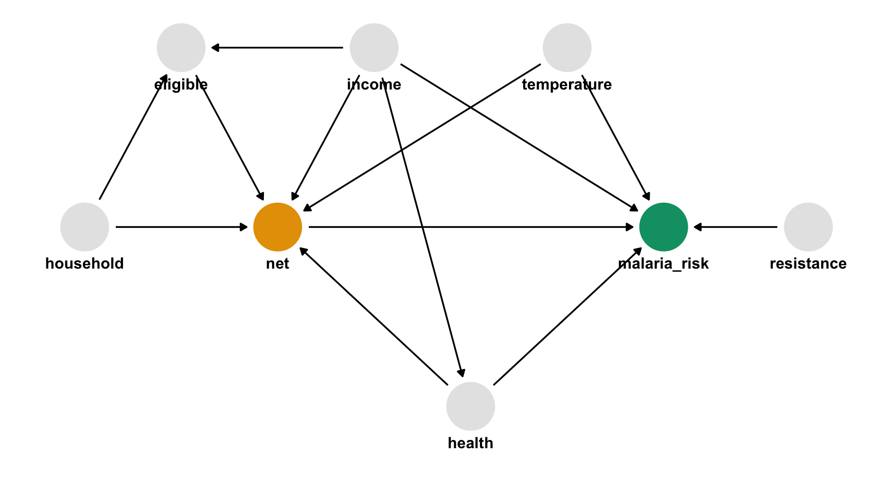
draw your assumptions
In words
- Malaria risk is causally impacted by net usage, income, health, temperature, and insecticide resistance.
- Net usage is causally impacted by income, health, temperature, eligibility for the free net program, and the number of people in a household.
- Eligibility for the free net programs is determined by income and the number of people in a household.
- Health is causally impacted by income.
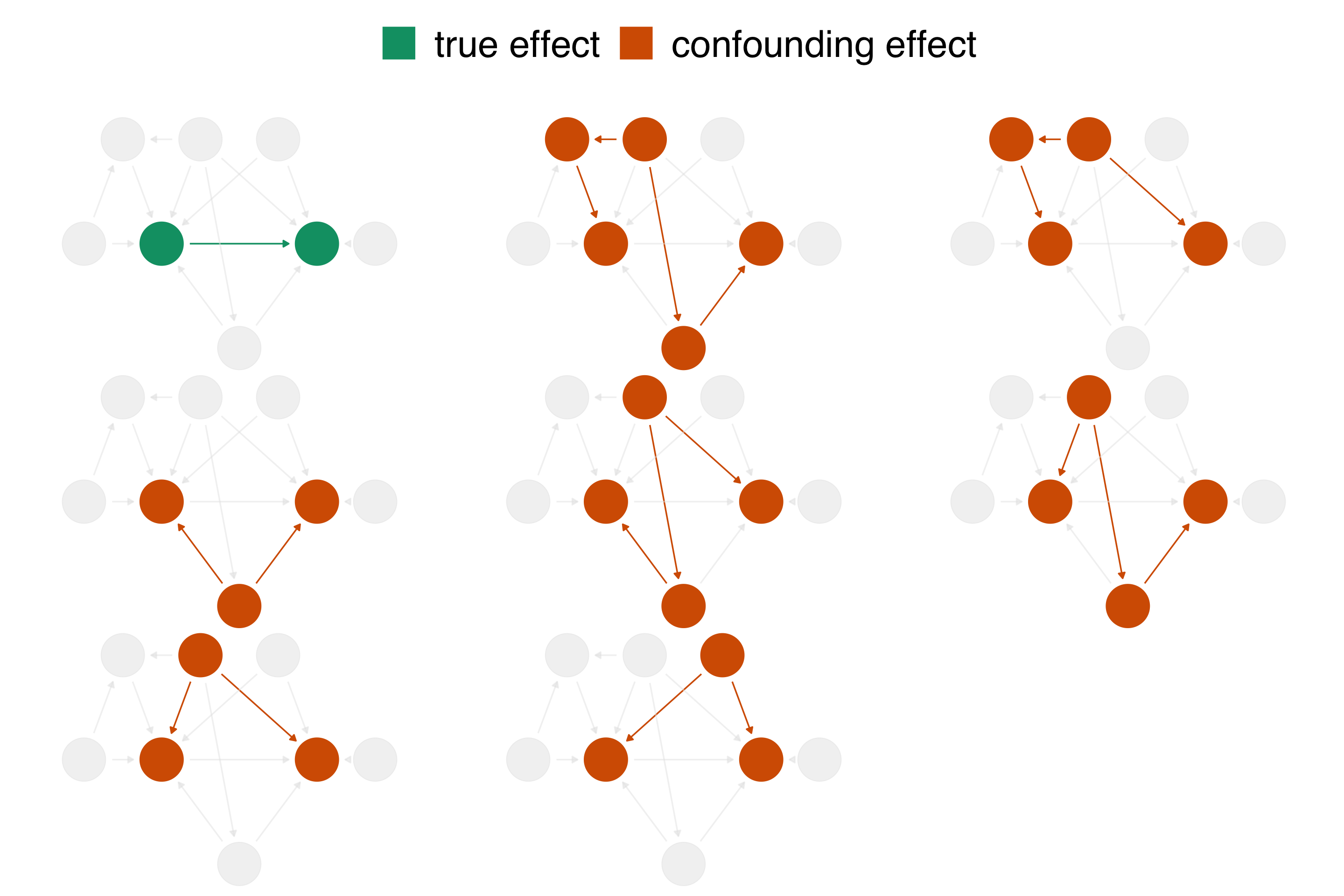
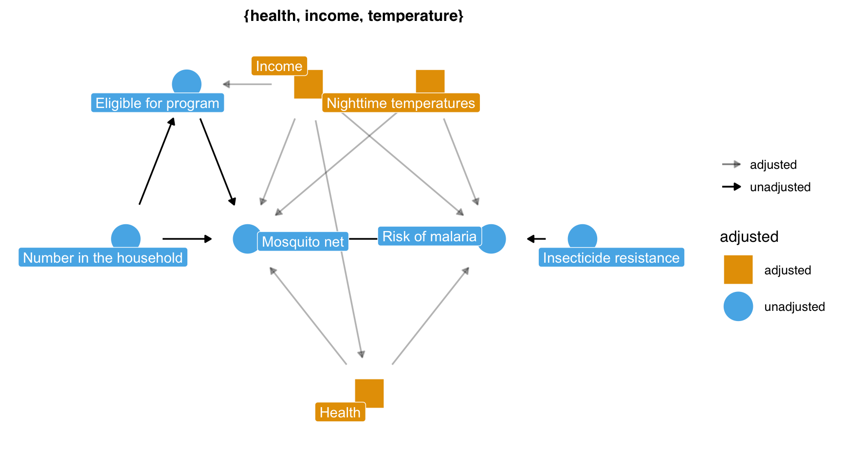
What do I need to control for?
Multivariable regression: what’s the association?
# A tibble: 1 × 7
  term    estimate std.error statistic   p.value
  <chr>      <dbl>     <dbl>     <dbl>     <dbl>
1 netTRUE    -12.0     0.314     -38.2 2.69e-232
  conf.low conf.high
     <dbl>     <dbl>
1    -12.6     -11.4
model your assumptions
counterfactual: what if everyone used a net vs. what if no one used a net
Fit propensity score model
Calculate inverse probability weights
library(broom)
library(propensity)
net_data_wts <- propensity_model |>
  augment(newdata = net_data, type.predict = "response") |>
  # .fitted is the value predicted by the model
  # for a given observation
  mutate(wts = wt_ate(.fitted, net))

net_data_wts |>
  select(net, .fitted, wts)
# A tibble: 1,752 × 3
net .fitted wts
<lgl> <dbl> <dbl>
1 FALSE 0.246 1.33
2 FALSE 0.218 1.28
3 FALSE 0.323 1.48
4 FALSE 0.231 1.30
5 FALSE 0.279 1.39
6 FALSE 0.306 1.44
7 FALSE 0.332 1.50
8 FALSE 0.168 1.20
9 FALSE 0.222 1.29
10 FALSE 0.255 1.34
# ℹ 1,742 more rowsdiagnose your model assumptions
What’s the distribution of weights?
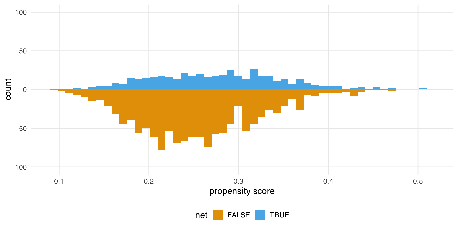
What are the weights doing to the sample?
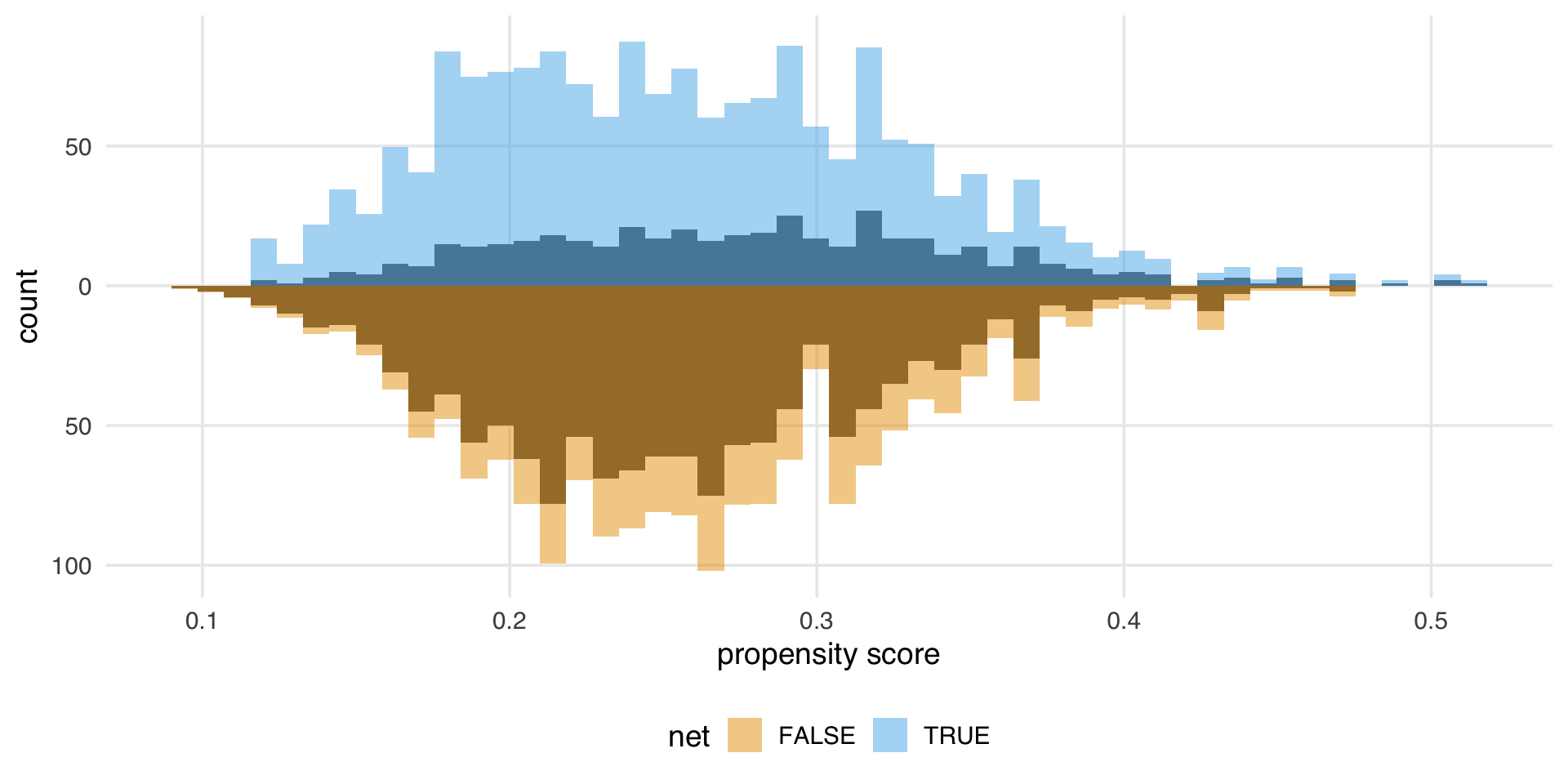
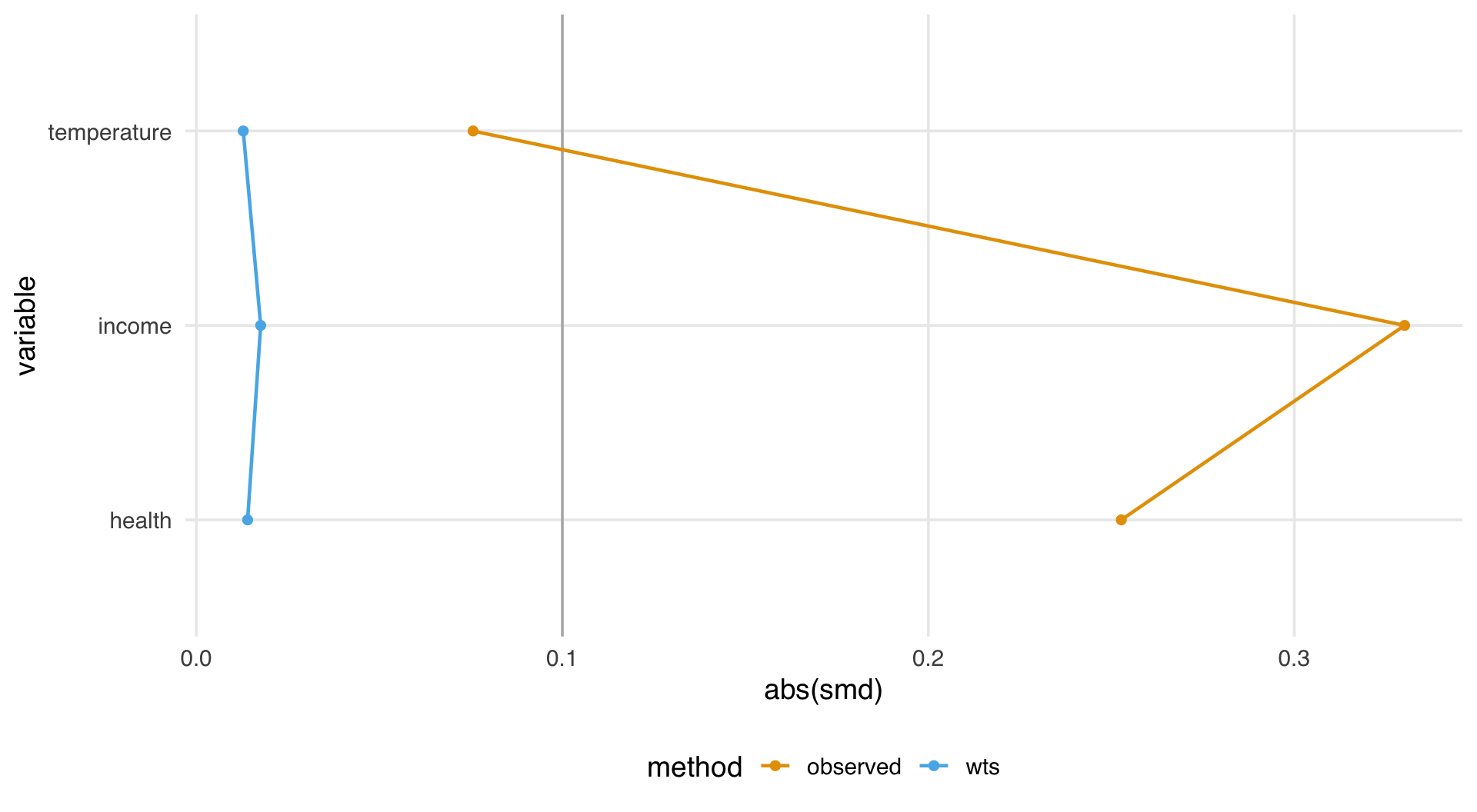
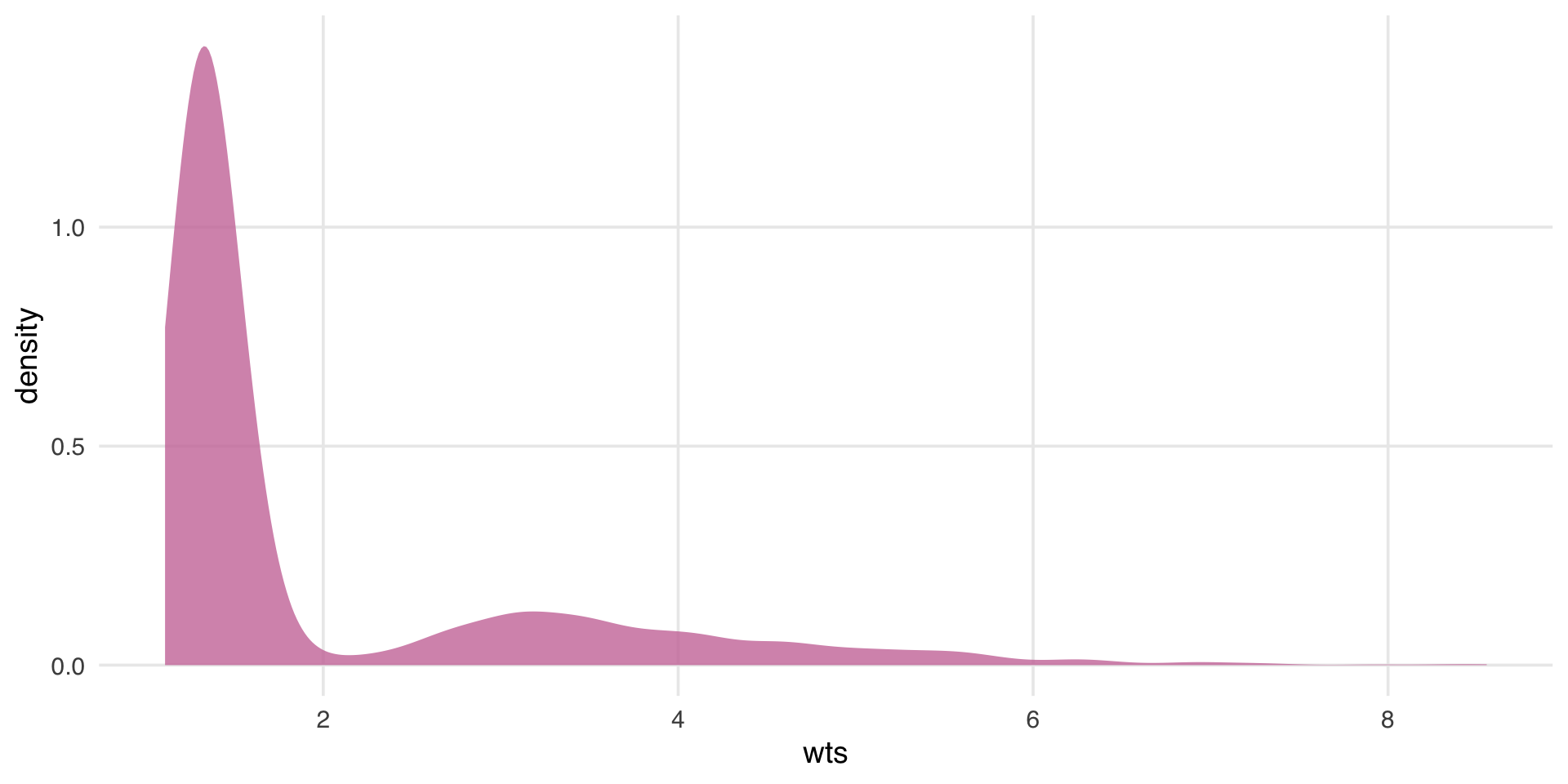
estimate the causal effects
Estimate causal effect with IPW
Estimate causal effect with IPW
Let’s fix our confidence intervals (robust SEs)!
Let’s fix our confidence intervals (robust SEs)!
Let’s fix our confidence intervals (bootstrap)!
fit_ipw <- function(split, ...) {
  .df <- analysis(split)

  # fit propensity score model
  propensity_model <- glm(
    net ~ income + health + temperature,
    family = binomial(),
    data = .df
  )

  # calculate inverse probability weights
  .df <- propensity_model |>
    augment(type.predict = "response", data = .df) |>
    mutate(wts = wt_ate(.fitted, net))

  # fit correctly bootstrapped ipw model
  lm(malaria_risk ~ net, data = .df, weights = wts) |>
    tidy()
}
Using {rsample}
Using {rsample}
Using {rsample}
# A tibble: 1 × 6
  term    .lower .estimate .upper .alpha .method
  <chr>    <dbl>     <dbl>  <dbl>  <dbl> <chr>
1 netTRUE  -13.4     -12.5  -11.7   0.05 student-t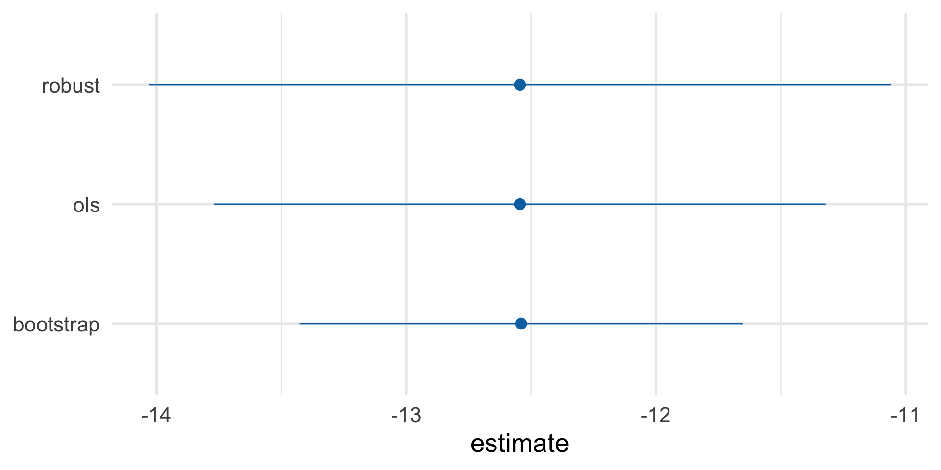
Our causal effect estimate: -12.5 (95% CI -13.4, -11.6)
sensitivity analysis
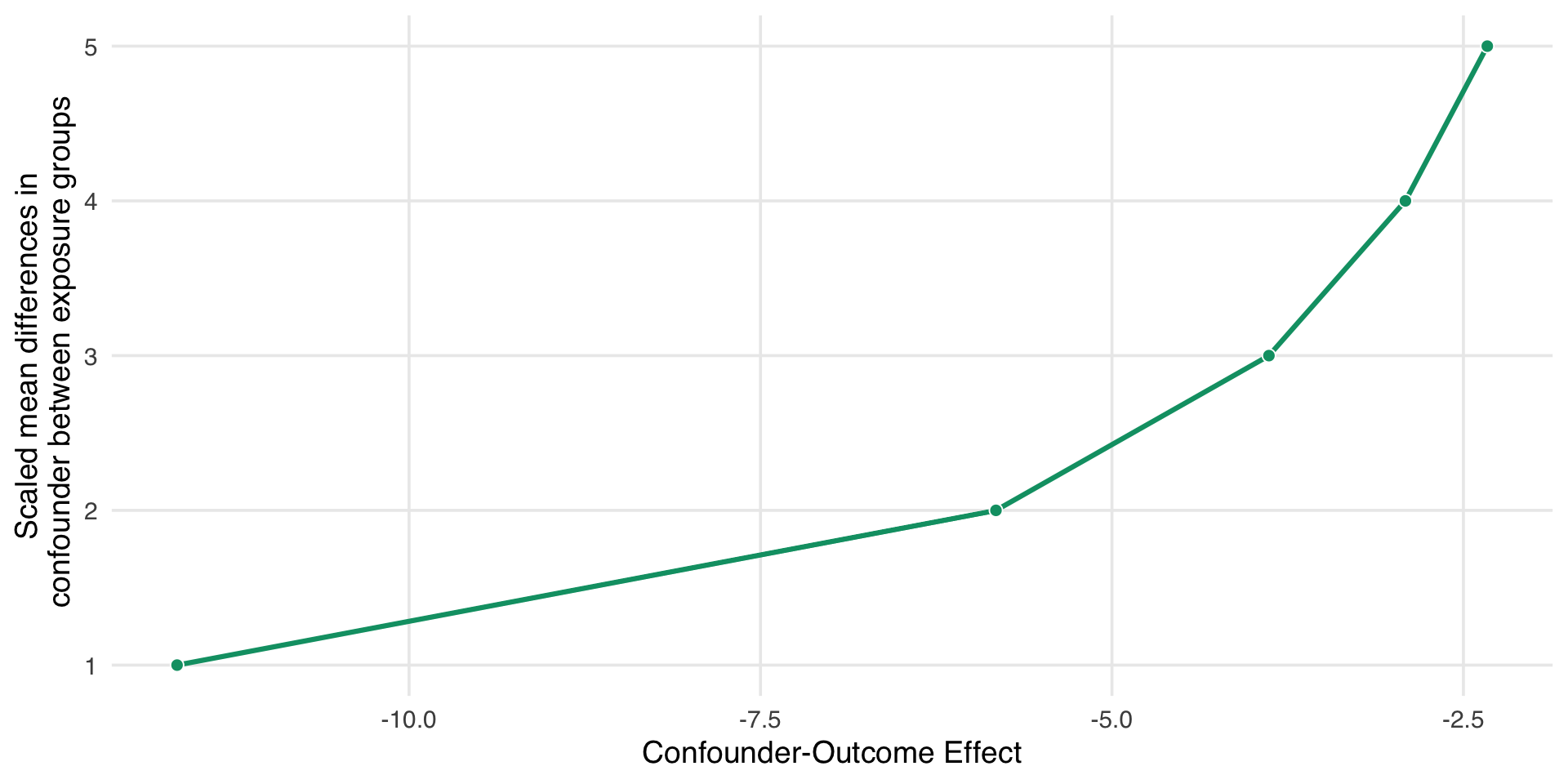
Sensitivity Analysis
More specific sensitivity analysis
- People with this genetic resistance have, on average, about 10 units lower malaria risk.
- About 26% of people who use nets in our study have this genetic resistance.
- About 5% of people who don’t use nets have this genetic resistance.
More specific sensitivity analysis
adjusted_estimates <- boot_estimate |>
  select(.estimate, .lower, .upper) |>
  unlist() |>
  adjust_coef_with_binary(
    exposed_confounder_prev = 0.26,
    unexposed_confounder_prev = 0.05,
    confounder_outcome_effect = -10
  )

adjusted_estimates
# A tibble: 3 × 4
effect_adjusted effect_observed
<dbl> <dbl>
1 -10.4 -12.5
2 -11.3 -13.4
3 -9.55 -11.7
exposure_confounder_effect confounder_outcome_effect
<dbl> <dbl>
1 0.21 -10
2 0.21 -10
3 0.21 -10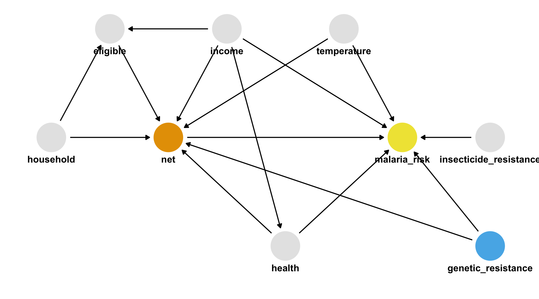
Truth
- The unmeasured confounder is in
net_data_fullas genetic_resistance. - If we recalculate the IPW estimate of the average treatment effect of nets on malaria risk, we get -10.2 (95% CI -11.2, -9.4), much closer to the actual answer of -10.
- Specified a causal question (for average treatment effect)
- Drew our assumptions using a causal diagram (using DAGs)
- Modeled our assumptions (propensity score weighting)
- Diagnosed our models (by checking confounder balance after weighting)
- Estimated the causal effect (using inverse probability weighting)
- Conducted sensitivity analysis on the effect estimate (using tipping point analysis)
Check out Chapter 2 of Causal Inference in R
Slides by Dr. Lucy D’Agostino McGowan
