Outcome Models

Lucy D’Agostino McGowan

Outcome Model (matching)

library(broom)
library(touringplans)
library(MatchIt)

m <- matchit(
  qsmk ~ sex + 
      race + age + I(age^2) + education + 
      smokeintensity + I(smokeintensity^2) + 
      smokeyrs + I(smokeyrs^2) + exercise + active + 
      wt71 + I(wt71^2),
  data = nhefs_complete_uc
)
matched_data <- get_matches(m, id = "i")

Outcome Model (matching)

lm(wt82_71 ~ qsmk, data = matched_data) |>
  tidy(conf.int = TRUE)

# A tibble: 2 × 7
  term        estimate std.error statistic  p.value conf.low
  <chr>          <dbl>     <dbl>     <dbl>    <dbl>    <dbl>
1 (Intercept)     1.05     0.397      2.63 8.61e- 3    0.267
2 qsmk            3.48     0.562      6.19 9.73e-10    2.37 
# ℹ 1 more variable: conf.high <dbl>

Application Exercise

10:00

Get starter files from https://github.com/sta-779-s25/appex-04-YOUR-GITHUB-HANDLE.git
Fit the propensity score matching model according to our DAG
Fit the outcome model to the matched data
Estimate the causal effect

Outcome Model (weighted)

library(broom)

lm(outcome ~ exposure, data = df, weights = wts) |>
  tidy()

✅ This will get us the point estimate

❌ This will get NOT us the correct confidence intervals

Estimating Uncertainty

Bootstrap
Sandwich estimator (on outcome model only)
Sandwich estimator (on outcome model + propensity score model)

1. Create a function to run your analysis once

(on a sample of your data)

fit_ipw <- function(split, ...) {
  .df <- analysis(split)
  
  # fit propensity score model
  propensity_model <- glm(
    qsmk ~ sex + 
      race + age + I(age^2) + education + 
      smokeintensity + I(smokeintensity^2) + 
      smokeyrs + I(smokeyrs^2) + exercise + active + 
      wt71 + I(wt71^2), 
    family = binomial(), 
    data = .df
  )
  
  # calculate inverse probability weights
  .df <- propensity_model |>
    augment(type.predict = "response", data = .df) |>
    mutate(wts = wt_ate(.fitted, qsmk, exposure_type = "binary"))
  
  # fit correctly bootstrapped ipw model
  lm(wt82_71 ~ qsmk, data = .df, weights = wts) |>
    tidy()
}

2. Use {rsample} to bootstrap our effect

library(rsample)

# fit ipw model to bootstrapped samples
bootstrapped_nhefs <- bootstraps(
  nhefs_complete_uc, 
  times = 1000, 
  apparent = TRUE
)

bootstrapped_nhefs

2. Use {rsample} to bootstrap our effect

# Bootstrap sampling with apparent sample 
# A tibble: 1,001 × 2
   splits             id           
   <list>             <chr>        
 1 <split [1566/583]> Bootstrap0001
 2 <split [1566/595]> Bootstrap0002
 3 <split [1566/577]> Bootstrap0003
 4 <split [1566/572]> Bootstrap0004
 5 <split [1566/565]> Bootstrap0005
 6 <split [1566/562]> Bootstrap0006
 7 <split [1566/555]> Bootstrap0007
 8 <split [1566/572]> Bootstrap0008
 9 <split [1566/579]> Bootstrap0009
10 <split [1566/570]> Bootstrap0010
# ℹ 991 more rows

2. Use {rsample} to bootstrap our effect

fit_ipw(bootstrapped_nhefs$splits[[1]])

# A tibble: 2 × 5
  term        estimate std.error statistic  p.value
  <chr>          <dbl>     <dbl>     <dbl>    <dbl>
1 (Intercept)     1.69     0.291      5.82 7.33e- 9
2 qsmk            3.73     0.410      9.09 2.87e-19

2. Use {rsample} to bootstrap our effect

ipw_results <- bootstrapped_nhefs |> 
  mutate(boot_fits = map(splits, fit_ipw)) 

ipw_results

2. Use {rsample} to bootstrap our effect

# Bootstrap sampling with apparent sample 
# A tibble: 1,001 × 3
   splits             id            boot_fits       
   <list>             <chr>         <list>          
 1 <split [1566/579]> Bootstrap0001 <tibble [2 × 5]>
 2 <split [1566/581]> Bootstrap0002 <tibble [2 × 5]>
 3 <split [1566/608]> Bootstrap0003 <tibble [2 × 5]>
 4 <split [1566/555]> Bootstrap0004 <tibble [2 × 5]>
 5 <split [1566/579]> Bootstrap0005 <tibble [2 × 5]>
 6 <split [1566/577]> Bootstrap0006 <tibble [2 × 5]>
 7 <split [1566/562]> Bootstrap0007 <tibble [2 × 5]>
 8 <split [1566/562]> Bootstrap0008 <tibble [2 × 5]>
 9 <split [1566/580]> Bootstrap0009 <tibble [2 × 5]>
10 <split [1566/602]> Bootstrap0010 <tibble [2 × 5]>
# ℹ 991 more rows

2. Use {rsample} to bootstrap our effect

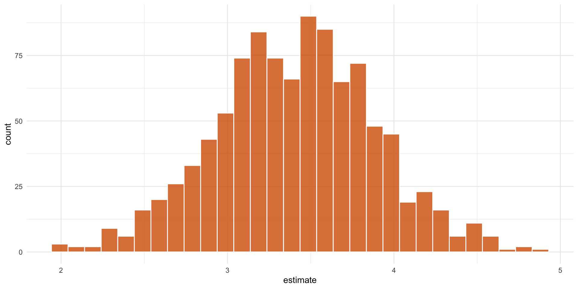
3. Pull out the causal effect

# get t-statistic-based CIs
boot_estimate <- int_t(ipw_results, boot_fits) |> 
  filter(term == "exposure")

Application Exercise

12:00

Create a function called ipw_fit that fits the propensity score model and the weighted outcome model for the effect between the exposure and outcome
Using the bootstraps() and int_t() functions to estimate the final effect.

Sandwich estimator

library(sandwich)
weighted_mod <- lm(wt82_71 ~ qsmk, data = nhefs_complete_uc, weights = wts)

sandwich(weighted_mod)

            (Intercept)        qsmk
(Intercept)  0.05050382 -0.05050382
qsmk        -0.05050382  0.27614347

Sandwich Estimator

robust_var <- sandwich(weighted_mod)[2, 2]
point_est <- coef(weighted_mod)[2]
lb <- point_est - 1.96 * sqrt(robust_var)
ub <- point_est + 1.96 * sqrt(robust_var)
lb

    qsmk 
2.410568

ub

    qsmk 
4.470503

Sandwich estimator with `{survey}`

library(survey)

des <- svydesign(
  ids = ~1,
  weights = ~wts,
  data = nhefs_complete_uc
)

Sandwich estimator with `{survey}`

svyglm(wt82_71 ~ qsmk, des) |>
  tidy(conf.int = TRUE)

# A tibble: 2 × 7
  term        estimate std.error statistic  p.value conf.low
  <chr>          <dbl>     <dbl>     <dbl>    <dbl>    <dbl>
1 (Intercept)     1.78     0.225      7.92 4.54e-15     1.34
2 qsmk            3.44     0.526      6.55 8.03e-11     2.41
# ℹ 1 more variable: conf.high <dbl>

Application Exercise

10:00

Use the sandwich package to calcualte the uncertainty for your weighted model
Repeat this using the survey package

Sandwich Estimator with `{propensity}`

This takes into account that you fit the propensity score model.

results <- ipw(propensity_model, weighted_mod)
results

Inverse Probability Weight Estimator
Estimand: ATE 

Propensity Score Model:
  Call: glm(formula = qsmk ~ sex + race + age + I(age^2) + education + 
    smokeintensity + I(smokeintensity^2) + smokeyrs + I(smokeyrs^2) + 
    exercise + active + wt71 + I(wt71^2), family = binomial(), 
    data = nhefs_complete_uc) 

Outcome Model:
  Call: lm(formula = wt82_71 ~ qsmk, data = nhefs_complete_uc, weights = wts) 

Estimates:
     estimate std.err       z ci.lower ci.upper conf.level   p.value    
diff   3.4405 0.48723 7.06145   2.4856   4.3955       0.95 1.648e-12 ***
---
Signif. codes:  0 '***' 0.001 '**' 0.01 '*' 0.05 '.' 0.1 ' ' 1

Sandwich Estimator with `{propensity}`

This takes into account that you fit the propensity score model.

results |> 
  as.data.frame()

  effect estimate   std.err        z ci.lower ci.upper conf.level      p.value
1   diff 3.440535 0.4872282 7.061446 2.485586 4.395485       0.95 1.647793e-12

Application Exercise

10:00

Use the {propensity} package to calcualte the uncertainty for your weighted model

Outcome Models

Outcome Model (matching)

Outcome Model (matching)

Application Exercise

Outcome Model (weighted)

Estimating Uncertainty

1. Create a function to run your analysis once

2. Use {rsample} to bootstrap our effect

2. Use {rsample} to bootstrap our effect

2. Use {rsample} to bootstrap our effect

2. Use {rsample} to bootstrap our effect

2. Use {rsample} to bootstrap our effect

2. Use {rsample} to bootstrap our effect

3. Pull out the causal effect

Application Exercise

Sandwich estimator

Sandwich Estimator

Sandwich estimator with {survey}

Sandwich estimator with {survey}

Application Exercise

Sandwich Estimator with {propensity}

Sandwich Estimator with {propensity}

Application Exercise

Sandwich estimator with `{survey}`

Sandwich estimator with `{survey}`

Sandwich Estimator with `{propensity}`

Sandwich Estimator with `{propensity}`